The Difference between Discrete & Continuous Variables

To understand the difference between discrete and continuous variables, we must first define what a random variable is:

Random Variable - a variable whose value is a numerical outcome of a random phenomenon. 

I. Continuous Random Variables

*You’ve seen them! Think normal distributions!

Continuous random variable - a variable (x) that can be any value within an interval of numbers

Examples:

height  (could range from 4 to 7 feet)

weight  (could range from 80 to 300 pounds)

time it takes to run a mile  (could range from 4 to 10 minutes)

Probability distribution of x is described by a density curve.  

Remember the density curve of a uniform distribution has a height 1 over the interval from 0 to 1. Area under the curve is 1.

With a continuous random variable, values are not isolated. Instead of a countable number of outcomes, each outcome is a different value. Therefore, rather than assigning probability to individual outcomes, probabilities are assigned to intervals.

In fact, individual outcomes have a probability of 0.

For the interval from 0 to 1 from .799-.901 the probability is .002; however, we can’t have an outcome exactly equal to .08. 

Example:

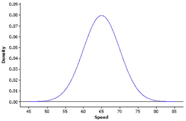
Suppose vehicle speeds at a highway location have a normal distribution with mean μ = 65 mph and standard deviation sd = 5 mph. The probability density function is shown below. Notice that the horizontal axis shows speeds and the bell is centered at the mean (65 mph).

What is the probability that the vehicle is traveling between 60 and 73 mpg at this particular highway location? 

P(60< X < 73) =

Z score for 60: \(z = {60-65 \over 5}\)=-1.00  →  p-value= .1587   

Z score for 73: \(z = {73-65 \over 5}\) = 1.6 → p-value= .9452

↓

P(60< X < 73) = 0.7875

The probability that the vehicle is traveling between 60 and 73 mpg at this particular highway location is 78.75%.

II. Discrete Random Variables

Discrete Random Variable - a variable (x) that has a countable number of possible values.

Examples:

flipping a coin  →  possible outcomes: heads or tails

rolling a dice  → posible outcomes: 1, 2, 3, 4, 5, or 6

grades  →  posible outcomes: A, B, C, D, or F

Probability distribution of random variable x lists the values and their probabilities.

Values of x:   x₁      x₂       x₃     …….    x_k

Probability:    p₁      p₂      p₃     ……..    p_k

The probabilities p_i must satisfy two requirements:

1. Every probability p_i is a number between 0 and 1.
2. p₁ + p₂ + p₃ + …. + p_k = 1 

*since there are limited number of potential values of x, it must be one of those values. Therefore, the summation of all the possible values of x is equal to 1 or 100%

Example: 

You toss a fair coin three times and record the outcomes. In particular you are concerned with the number of heads. 

x= number of heads

Possible outcomes:

TTT: x=0

HTT, THT, TTH: x=1

HHT, HTH, THH: x=2

HHH: x=3

Number of possible outcomes= 8 (This can also be thought of as 2³ → 2 options repeated 3 times)

Probability of each possible outcomes: 

P(x=0) = 1/8 = .125

P(x=1) = 3/8 =  .375

P(x=2) = 3/8 = .375

P(x=3) = 1/8= .125

Note: both requirements are satisfied as the probability of each event is between 0 and 1 and the sum of all the outcome probabilities is equal to 1.

In addition to being able to find the percent of an individual outcomes you can also find the probability of multiple outcomes

Examples:

the probability of getting two or more heads:

P(x≥2) = P(x=2) + P(x=1) + P(x=0)= .375 + .25 + .0625 = .6875

the probability of getting 1 or more heads:

*Use the complement rule

P(x≥1) = 1- P(x=0) = 1 - .0625 = .9375