Inference for Linear Regression
Introduction
Let's say that you are analyzing the relationship between two variables. You take several samples and create a least squares regression line for each. The image below shows these least square regression lines generated from different random samples as solid grey lines, and the true population regression line as a dotted blue line. Notice how the grey lines all “estimate” the slope and intercept of the true regression line.
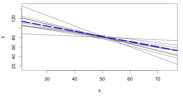
The least squares regression line (\(\widehat {y} = a + bx\)), which runs through a sample of data points, is really an estimate of the true population regression line (\(\mu_y = \alpha + \beta x\)). Just like we use sample statistics to estimate population parameters, we can use \(a\) and \(b\) to perform hypothesis tests and construct confidence intervals to estimate the values of \(\alpha\) and \(\beta\).
We conduct statistical inference in linear regression when we find a sample slope and then use it to make a confidence interval or perform a hypothesis test about the true population slope.
Confidence Interval
When you construct a confidence interval for the slope of a LSRL (\(b\)), you are creating a range of values, within which you hope lies the true population slope (\(\beta\)).
* SEb refers to the standard error of \(b\).
Hypothesis Test
When you run a hypothesis test for the slope of a LSRL, you test to see if there is...
- any association between the two variables ( \(\beta \neq 0\) )
- a positive association between the two variables ( \(\beta > 0\) )
- or a negative association between the two variables ( \(\beta < 0\) )
Most of the time, \(H_0: \beta = 0\) will be our null hypothesis. It suggests that there is not linear relationship between x and y. If we are able to prove this wrong, we can get good evidence to suggest that we do have a linear relationship. With this in mind, we can now define the test as follows:
\(H_0: \beta = 0\) (no association)
\(H_A: \) \(\beta \neq 0\), \(\beta > 0\), or \(\beta < 0\)
Because \(\beta = 0\), the formula can be simplified as follows:
* SEb refers to the standard error of \(b\).
Degrees of Freedom
Where \(n\) is the sample size:
Conditions for Performing Inference About the Linear Regression Model
1. The observations are independent (individual observations don’t affect other observations).
2. The data comes from a random sample.
3. The response variable is roughly linear with x.
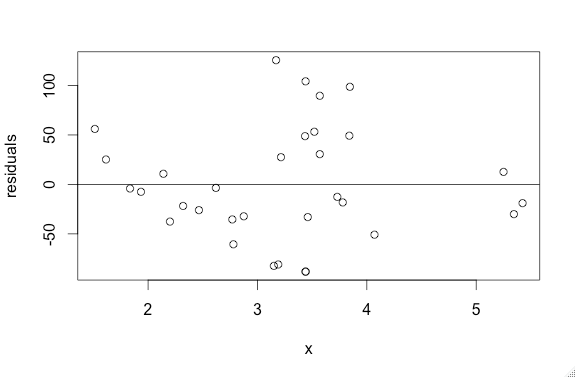
4. The standard deviation (SEb) of the y-variable is the same for all values x.
You can easily check this by looking at the graph of the residual. If the spread of the residuals changes along the x axis, then the standard deviation is changing and you cannot use the data.
5. The least-squared regression lines vary normally about the true regression line.
Interpreting Tables
You may be wondering where you find SEb . This value is given in a table.
In problems when you are asked to conduct statistical inference for linear regression, you will be given tables like the following (with different numbers depending on the scenario):
| Predictor | Estimate | Standard Error | t | p |
| Constant (Intercept) | -3.06 | 1.6 | -1.9 | 0.2 |
| Variable x (Slope) | 1.94 | 0.493 | 3.93 | 0.027 |
Let's break it down:
- The "Constant" refers to the y-intercept, and the "Variable x" refers to the slope. You will usually conduct inference for the slope, so we will focus exclusively on the "Variable x" for now.
- The "Estimate" refers to the point estimate (\(b\)), and will be used in the formulas for confidence intervals and hypothesis tests.
- The "Standard Error" refers to SEb, and will also be used in the formulas for confidence intervals and hypothesis tests.
- The next two columns are not always included on the table, because sometimes it is your job to find those values.
- "t" refers to the test statistic you get from calculating the hypothesis test formula (\(t = {b \over SE_b}\)).
- "p" refers to the p-value you get after running your test statistic through the tcdf function on your calculator. Note that the given p-value is always for a 2-sided test (\(\beta \neq 0\)).
Sample Problem
Catherine is studying the relationship between club participation and free time among the students at her school. She randomly selects 26 students and asks them to submit the number of clubs they are registered with and the average hours of free time they have per night. She then compiles the data and finds the least squares regression line. Below is the computer output from her LSRL:
|
Predictor |
Coef |
StDev |
t |
p |
|
Constant |
5.67 |
3.46 |
1.638 |
0.114 |
|
Clubs Joined |
-2.12 |
0.78 |
-2.72 |
0.012 |
Remember: Before you can continue on, you MUST CHECK THE CONDITIONS outlined above.
A) Confidence Interval: Construct an 80% confidence interval for this data.
1. Calculate the interval using the formula \(b ^+_- (t^*)(SE_b)\) .
i. Find the degrees of freedom: \(n - 2\) = \(26 - 2\) = 24
ii. Find the t* value using a t-table: 1.3178
ii. \(b ^+_- (t^*)(SE_b)\) → \((-2.12) ^+_- (1.3178)(0.78)\) → \((-2.12) ^+_- (1.0279)\)
→ \((-2.12) + (1.0279) = -1.0921\)
→ \((-2.12) - (1.0279) = -3.1479\)
Final Interval: (-3.1479, -1.0921)
2. State your conclusion.
Based on the data, I am 80% confident that students' number of hours of free time decreases by between 3.1479 and 1.0921 for every additional club they are a member of.
B) Hypothesis Test: Conduct a hypothesis test to see if there’s a linear relationship between the number of clubs one has joined and hours of free time one has.
1. Define the test.
\(H_0: \beta = 0\) (the number of clubs joined has no effect on the number of hours of free time)
\(H_A: \beta < 0\) (the number of clubs joined has a negative effect on the number of hours of free time)
2. Find the test statistic from the computer output or using the formula (** it is important to be able to do this both ways becauase sometimes the tables will not include "t" and "p").
i. Computer output: t = -2.72
ii. Formula: \(t = {b \over SE_b}\) → \(t = {-2.12 \over 0.78} = -2.72\)
3. Find the p-value from the computer output or the tcdf function on your calculator.
i. Computer output: 0.006
Remember that the p-value displayed on the table is for a TWO-sided test. However, we want to conduct a ONE-sided test. This means that you have to divide the given p-value by 2 → \(0.012 \div 2 = 0.006\)
ii. Calculator:
In the tcdf function of your calculator, input your lower limit (-999), your upper limit (-2.72), and the degrees of freedom (24). The calculator should produce 0.006.
4. State your conclusion.
I calculated a p-value of 0.006, which is less than the standard assumed significance level of 0.05. Therefore, we REJECT the null hypothesis. Our data supports the claim that the number of clubs a student is a member of has a negative effect on his or her hours of free time.