STATS4STEM

R: Boxplot

I. Basic Boxplot
An electric car manufacturer asked engineers to do nine seperate endurance tests on two of their car models. One model is called the Electra and the second is called the

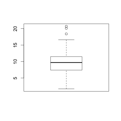
# create wind variable to be used to construct boxplots
wind = airquality$Wind

boxplot(wind)

II. horizontal and col parameters
An electric car manufacturer asked engineers to do nine seperate endurance tests on two of their car models. One model is called the Electra and the second is called the

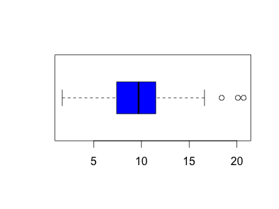
boxplot(wind, 
        horizontal = TRUE, 
        col = "blue")

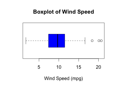
III. main and xlab parameters
An electric car manufacturer asked engineers to do nine seperate endurance tests on two of their car models. One model is called the Electra and the second is called the

boxplot(wind, 
        horizontal = TRUE, 
        col = "blue", 
        main = "Boxplot of Wind Speed",
        xlab = "Wind Speed (mpg)")

IV. Side-by-side Boxplots
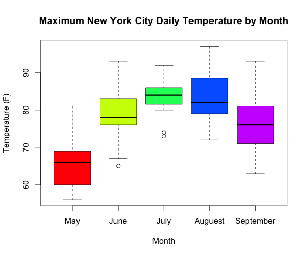
Side-by-side boxplots are an excellent graphical tool to help discern the relationship between a categorical and numerical variables.

Example 1:

For this example, we will use the preinstalled airquality dataset that contains data for New York City. For this specific example we will be analyzing the relationship between the maximum New York City daily temperature and month. Before we can begin our analysis, for simplicity, we first will define two new variables as shown below.

temp = airquality$Temp
month = airquality$Month

Next, let's analyze the relationship between maximum daily temperature and month. To do this, we will construct a side-by-side boxplots using the R code shown below:

boxplot(temp ~ month,  
        col = rainbow(5),   
        names = c("May", "June", "July", "Auguest", "September"),
        main = "Maximum New York City Daily Temperature by Month",  
        xlab = "Month",   
        ylab = "Temperature (F)")

Example 2:

For this example, we will use the cats dataset found in the MASS library. To access this dataset, we will first need to load the MASS library first. Once the library has been loaded, one can view a small portion of the dataset, to get a feel for the dataset, by using the head(cars) command as shown below.

> # Load MASS library
> library(MASS)
> 
> head(cats)
  Sex Bwt Hwt
1   F 2.0 7.0
2   F 2.0 7.4
3   F 2.0 9.5
4   F 2.1 7.2
5   F 2.1 7.3
6   F 2.1 7.6

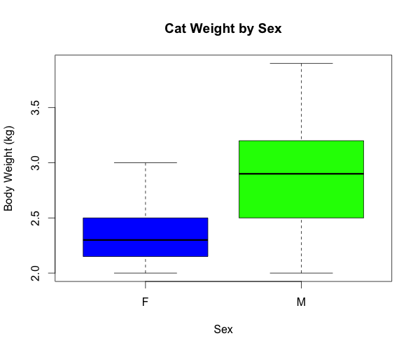
Once the data has been loaded, let's analyze the relationship between sex and body weight, which is represented by the Bwt variable. To do this, we will construct a side-by-side boxplot using the R code shown below:

# define two variables to be analyzed in boxplot
sex = cats$Sex
weight = cats$Bwt

boxplot(weight ~ sex,
        col = c("blue", "green"),
        main = "Cat Weight by Sex",
        xlab = "Sex",
        ylab = "Body Weight (kg)")

This work is licensed under a Creative Commons Attribution-NonCommercial-ShareAlike 4.0 International License.