R: Linear Regression - Basic

The following data represents the trunk width and tree height of 10 randomly chosen maple trees from Leominster State Forest.

Using the data above:
a) Enter the data in into R.
b) Construct a scatterplot with fitted least-squares regression line
c) Calculate the correlation and equation of the least-squares regression line
d) Construct a residual plot

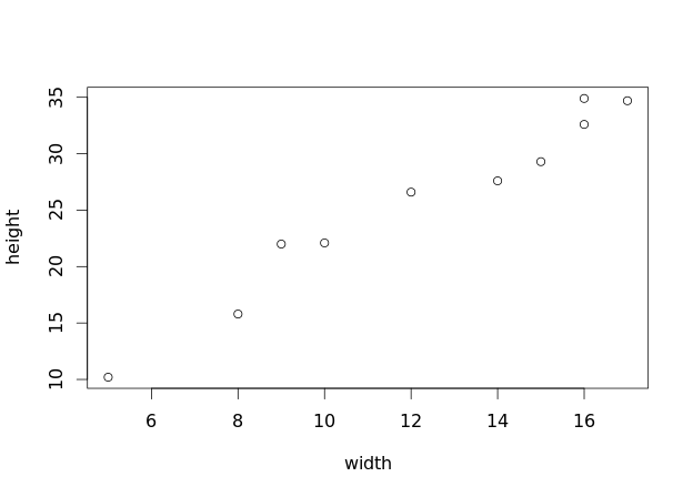
I. Enter Data & Construct Scatterplot

Begin by entering the data into R and then construct a scatterplot:

width = c(12, 15, 5, 17, 8, 10, 14, 16, 16, 9)
height = c(26.6, 29.3, 10.2, 34.7, 15.8, 22.1, 27.6, 34.9, 32.6, 22.0)

plot(width, height)

II. Construct Least-Squares Regression Model

After inspecting the scatterplot, it appears as though a linear regression model may be a good choice. We will use the lm(y.variable.name ~ x.variable.name) function. Once we create the model in R, and give it a variable name, if we call on the variable name, the y-intercept and slope will be provided. 

> model = lm(height ~ width)
> model

Call:
lm(formula = height ~ width)

Coefficients:
(Intercept)        width  
      1.557        1.969  

From the output we know that the equation for the least-squares regression:

\(\hat{y} = 1.557 + 1.969x\)

III. Calculate Correlation

Use the cor(x.variable, y.variable) function to calculate the correlation between the two variables.

> cor(width, height)
[1] 0.9804134

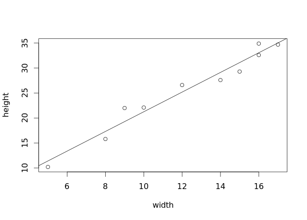
IV. Add Least-Squares Regression Line to Scatterplot

Now that we have constructed the scatterplot, and built and labeled the least-squares regression model, let's add the least-squares regression line to the scatterplot using the abline(model.name) function. Note: To perform the next step, you must have first constructed the scatterplot as shown in section I above.

abline(model)

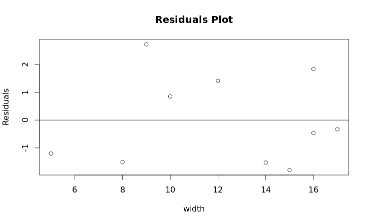
V. Construct Residuals Plot

Next we will use the resid(model.name) function to calculate the residuals. Once we have the residuals, we will then construct a residual plot using the plot() and abline() functions. Note: We will use abline(h = 0) to construct a horizontal line on our plot at y = 0. 

> # CALCULATE RESIDUALS
> r = resid(model)
> r
         1          2          3          4          5          6          7 
 1.4138211 -1.7934959 -1.2024390 -0.3317073 -1.5097561  0.8520325 -1.5243902 
         8          9         10 
 1.8373984 -0.4626016  2.7211382 
> 
> # CONSTRUCT RESIDUAL PLOT
> plot(width, r,
+      ylab = "Residuals",
+      main = "Residuals Plot")
> 
> # ADD HORIZONTAL LINE AT RESIDUALS = 0
> abline(h = 0)

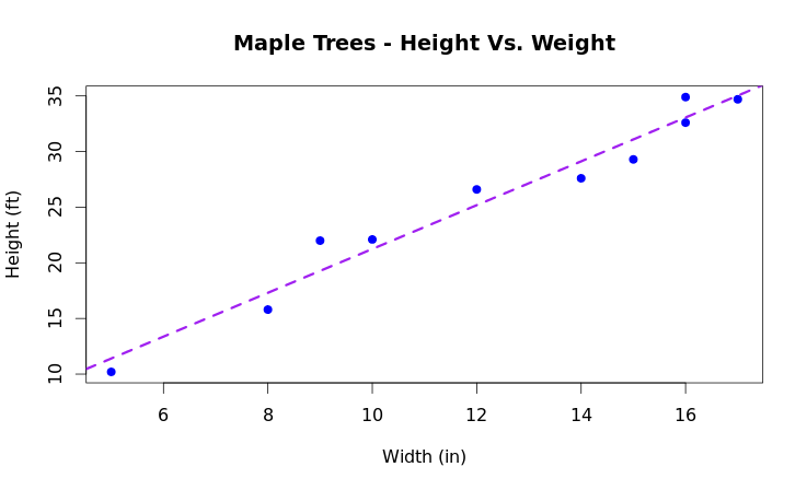
VI. (OPTIONAL) Make Graphs Prettier :)

Once you have constructed your graphs, you may wish to go back and make them more appealing to look at with different colors, line types, symbols, etc. The following is an example of how to do this.

plot(width, height,
     xlab = "Width (in)",
     ylab = "Height (ft)",
     main = "Maple Trees - Height Vs. Weight",
     pch = 19,
     col = "blue")

# ADD LEAST-SQUARES REGRESSION LINE TO YOUR GRAPH
abline(model,
       lty = 2,
       lwd = 3,
       col = "purple")

This work is licensed under a Creative Commons Attribution-NonCommercial-ShareAlike 4.0 International License.