R - Exponential Growth Modeling
Exponential Example A
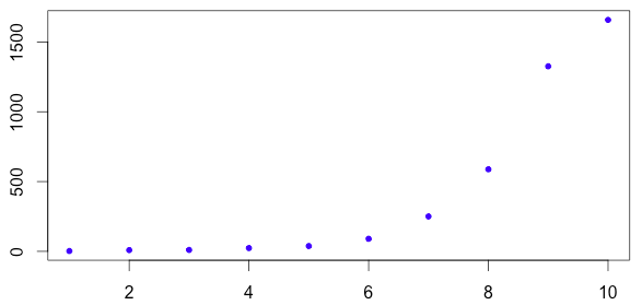
The data set is x=(1, 2, 3, 4, 5, 6, 7, 8, 9, 10) and y=(2.4, 8.8, 9.9, 23.5, 38.1, 90.1, 250.1, 587.9, 1325.7, 1658.3)
Store the data under the variables "x" and "y"
x=c(1, 2, 3, 4, 5, 6, 7, 8, 9, 10)
y=c(2.4, 8.8, 9.9, 23.5, 38.1, 90.1, 250.1, 587.9, 1325.7, 1658.3)
If these points are plotted the exponential nature of the data is evident, as seen below
For this exponential model take the log of the y values, and store it under a random variable, "ly"
ly=log10(y)
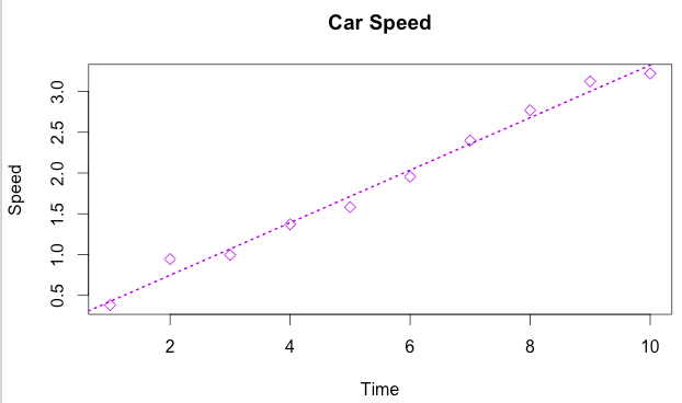
Plot the new graph, using the "x" and "ly" points
plot(x, ly,
     col="purple",
     pch=5,
     xlab="Time",
     ylab="Speed",
     main="Car Speed")
Create the line of best fit for the exponential model, stored under the variable "model"
model=lm(ly~x)
Add the line to the graph
abline(model,
       col="purple",
       lty=3,
       lwd=2)
The final code is below
x=c(1, 2, 3, 4, 5, 6, 7, 8, 9, 10)
y=c(2.4, 8.8, 9.9, 23.5, 38.1, 90.1, 250.1, 587.9, 1325.7, 1658.3)
ly=log10(y)
plot(x, ly, col="purple", pch=5, xlab="Time", ylab="Speed", main="Car Speed")
model=lm(ly~x)
abline(model, col="purple", lty=3, lwd=2)
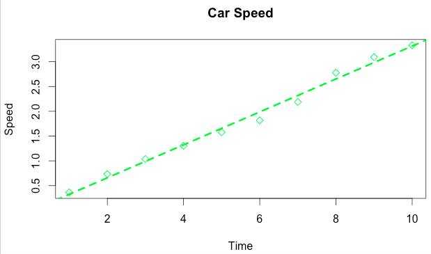
This is the new graph
Exponential Example B
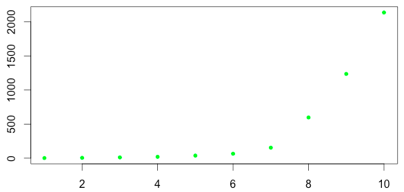
The data set is x=(1, 2, 3, 4, 5, 6, 7, 8, 9, 10) and y=(2.3, 5.4, 10.9, 20.0, 37.7, 65.4, 153.8, 597.4, 1236.2, 2137.0)
Store the data under the variables "x" and "y"
x=c(1, 2, 3, 4, 5, 6, 7, 8, 9, 10)
y=c(2.3, 5.4, 10.9, 20.0, 37.7, 65.4, 153.8, 597.4, 1236.2, 2137.0)
If these points are plotted the exponential nature of the data is evident, as seen below
For an exponential model take the log of the y values, and store it under a random variable, here "lgy"
lgy=log10(y)
Plot the new graph, using the "x" and "ly" points
plot(x, lgy,
     main="Car Speed",
     xlab="Time",
     ylab="Speed",
     pch=5,
     col="green2")
Create the line of best fit for the exponential model, stored under the variable "tr"
tr=lm(ly~x)
Add the line to the graph
abline(tr,
       col="green2",
       lwd=3,
       lty=2)
The final code is below
x=c(1, 2, 3, 4, 5, 6, 7, 8, 9, 10)
y=c(2.3, 5.4, 10.9, 20.0, 37.7, 65.4, 153.8, 597.4, 1236.2, 2137.0)
lgy=log10(y)
plot(x, lgy, main="Car Speed", pch=5, xlab="Time", ylab="Speed", col="green2")
tr=lm(ly~x)
abline(tr, col="green2", lwd=3, lty=2)
This is the new graph