R - Power Law Model

I. Introduction

A traditional linear model takes the form of \(\hat{y} = a + bx\). The power law model can be used in certain instances where the data appears nonlinear when plotting the response variable against the explanatory variable.  To implement the power law, the \(x\) and \(y\) variables need to be tranformed to \(log(x)\) and \(log(y)\). Once the transformation has been done, the transformed data should appear to be linear when plotted against each other on a scatterplot. 

II. Example

The following dataset below will be used to model the power law. 

GRAPH DATA

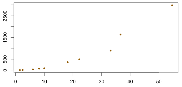
Lets begin by graphing our data, to do this, we must first store the data under "x" and "y" variables

x = c(1.49, 2.46, 6.05, 8.17, 9.97, 18.17, 22.20, 33.12, 36.60, 54.60)
y = c(2.01, 6.05, 33.12, 66.69, 81.45, 365.04, 492.75, 897.85, 1635.98, 2980.96)

If these points are plotted, it becomes evident that the data is non-linear as seen below. 

CHOOSE APPROPRIATE MODEL

Now that we know the data is clearly non-linear, one must determine if either the exponential growth or power law models can adequately be used to model the data. One easy way to quickly determine which model may be better is to calculate \(r^{2}\)for both methods. This analysis is shown below, and one can clearly see that \(r^{2} = 0.81\) for the exponential growth model, and \(r^{2} = 0.99\) for the power law model. Therefore, we will continue our analysis under the assumption that the power law model is more appropriate for this dataset.

> # Define Transformations
> lx = log10(x)
> ly = log10(y)
> 
> # r-squared - Exponential Growth
> cor(x, ly)^2
[1] 0.8095691
> # r-squared - Power Law
> cor(lx, ly)^2
[1] 0.997505

MODEL DATA USING POWER LAW

Create the line of best fit for the power law model, stored under the variable "model"

model = lm(ly ~ lx)

PLOT DATA USING POWER LAW

Plot the new graph, using the "lx" and "ly" points

plot(lx, ly,
     xlab="log(x)", 
     ylab="log(y)", 
     main="Power Law Graph", 
     pch=18, 
     col="gold2")

Add the line to the graph

abline(model, 
       col="gold2", 
       lty=6, 
       lwd=2)

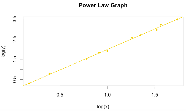
This is the new graph

DETERMINE POWER LAW FORMULA

Now that we see that model is a good fit, we can determine the mathematical equation to best model the data.

> model

Call:
lm(formula = ly ~ lx)

Coefficients:
(Intercept)           lx  
   -0.04408      2.02907  

Based on the R output above, we know the equation to be:

\(log(\hat{y}) = -0.441log(x) + 2.0291\)

Now, if we solve for \(\hat{y}\) we get:

\(10^{log(\hat{y})} =10^{ -0.441log(x) + 2.0291}\)

Simplifying further, we get:

\(\hat{y} = 10^{ -0.441log(x) + 2.0291}\)

MAKE PREDICTION USING POWER LAW FORMULA AND CHECK WORK

Now we can use the model above to make predictions. Lets use the formula from above to calculate \(\hat{y}\) when \(x = 30.\)

> x=30
> yhat = 10^(2.0291*log10(x) + 0.0441)
> yhat
[1] 1099.833

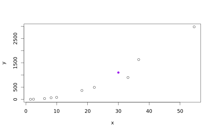
From the output, we can see that the  \(\hat{y} = 1099.83\) when \(x = 30.\) Now, lets plot the new predicted point on our original scatterplot to ensure that the prediction is valid, and our work was done correctly.

x=c(1.49, 2.46, 6.05, 8.17, 9.97, 18.17, 22.20, 33.12, 36.60, 54.60)
y=c(2.01, 6.05, 33.12, 66.69, 81.45, 365.04, 492.75, 897.85, 1635.98, 2980.96)
plot(x,y)

# PLOT PREDICTED POINT
points(30, 1099.83, col = "purple", pch = 16)

As one can see above, the predicted value fits the data very well. Job well done. 

x=c(1.49, 2.46, 6.05, 8.17, 9.97, 18.17, 22.20, 33.12, 36.60, 54.60)
y=c(2.01, 6.05, 33.12, 66.69, 81.45, 365.04, 492.75, 897.85, 1635.98, 2980.96)
plot(x,y)

# Define Transformations
lx = log10(x)
ly = log10(y)

# r-squared - Exponential Growth
cor(x, ly)^2
# r-squared - Power Law
cor(lx, ly)^2

plot(lx, ly, xlab="log(x)", ylab="log(y)", main="Power Law Graph", pch=18, col="gold2")
model=lm(ly~lx)
abline(model, col="gold2", lty=6, lwd=2)
model
yhat = (10^(-0.0441))*(x^2.0291)
yhat

x=c(1.49, 2.46, 6.05, 8.17, 9.97, 18.17, 22.20, 33.12, 36.60, 54.60)
y=c(2.01, 6.05, 33.12, 66.69, 81.45, 365.04, 492.75, 897.85, 1635.98, 2980.96)
plot(x,y)

# PLOT PREDICTED POINT
points(30, 1099.83, col = "purple", pch = 16)