STATS4STEM

R: Normal Distribution

I. Calculating P(X < x)
If X~N(μ, σ), use the pnorm(x, μ, σ) function to calculate P(X < x).

Example 1.a:

If X~N(85, 5), use the following R code to calculate P(X < 81).

> pnorm(81, 85, 5)
[1] 0.2118554

Example 1.b:

If X~N(85, 5), use the following R code to calculate P(X < 81). This method involves first calculating z, then using the pnorm function to find the area to the left of z using the standard normal distribution.

> # Calculate z
> z = (81 - 85)/5
> z
[1] -0.8
> 
> # define standard normal
> pnorm(z, 0, 1)
[1] 0.2118554
> 
> # if the mean and sd not provided,
> # R assumes mean = 0, sd = 1
> pnorm(z)
[1] 0.2118554

II. Calculating P(X > x)

If X~N(μ, σ), use the pnorm(x, μ, σ, lower.tail = FALSE) function to calculate P(X > x). A second method would be to subtract pnorm(x, μ, σ) from 1.

Example 1:

If X~N(85, 5), use the following R code to calculate P(X > 81).

# Method 1 - Use "lower.tail = FALSE"
> pnorm(81, 85, 5, lower.tail = FALSE)
[1] 0.7881446

# Method 2 - Subtract pnorm(x, n, p) from 1
> 1 - pnorm(81, 85, 5)
[1] 0.7881446

III. Given percentile, find corresponding x-value

If X~N(μ, σ), use the qnorm(percentile, μ, σ) function to find the x-value that corresponds with a given percentile.

Example 1:

If X~N(30, 3), what x-value corresponds with the 75th percentile?

> qnorm(0.75, 30, 3)
[1] 32.02347

Example 2: Jetblaster is a popular game app. Scores on the game are normally distributed with a mean of 1,114 and a stanard deviation of 321. Jack wishes to qualify for the national tournament. Only those who have a score in the top 10% qualify. What is the minimum score Jack needs to qualify for the national tournament? (Hint: The 90th percentile is the cutoff to score in the top 10 percent.)

> qnorm(0.9, 1114, 321)
[1] 1525.378

IV. Simulating Normal Random Variables
In statistics, one often finds the need to simulate random scenarios that are normally distributed. To do this, we need to use the rnorm(n, μ, σ) function, where n represents the number of random observations you wish to observe.

Example 1:

Scores on the Jetblaster app game are normally distributed with a mean of 1,114 and a stanard deviation of 321. Simulate 8 random scores of this game.

> rnorm(8, 1114, 321)
[1]  976.8647 1294.5687  512.8734  931.0832
[5] 1286.8615 1076.7246 1020.6694 1414.6181

Conclusion: The above code simulated 8 Jetblaster game scores. As one can interpret from the results, the first score was 976.8647, and the second score was 1294.5687.

IV. Assessing Normality
Often one must try to assess if data is actually normally distributed. There are a few methods available to do this. One very popular method is to construct a normal probability plot.

Example 1:

Sample 1000 observations from a normally distributed random variable that has a mean of 30 and a standard deviation of 3. Then construct a histogram and normal probability plot to assess normality.

# Randomly sample 1000 observations from N(30, 3)
data = rnorm(1000, 30, 3)

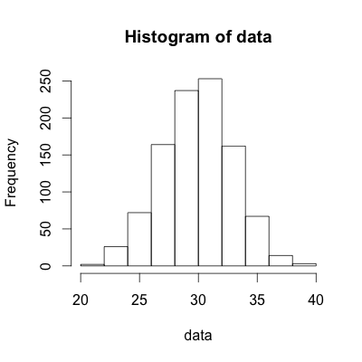
# Construct histogram
hist(data)

# Construct Normal Probability Plot
qqnorm(data, main = "Normal Probability Plot")

# Add diagonal line to help with normality assessment
qqline(data)

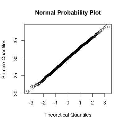Conclusion: As one would expect given that the data was drawn from the normal distribution, the histogram clearly looks to be normally distributed. Upon inspection of the Normal Probability Plot, one can see that the points line up with the line. When the points line up well with the horizontal line, one can assume the data is normally distributed, as is the case shown above.

This work is licensed under a Creative Commons Attribution-NonCommercial-ShareAlike 4.0 International License.