Sampling Distributions - Means
I. Introduction
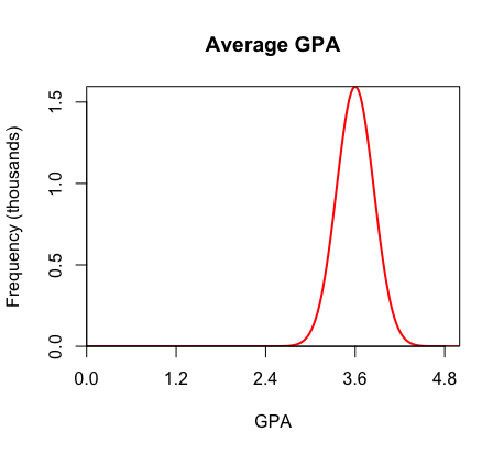
Imagine that there is a population of students at a large high school with a mean GPA of 3.6. You do not know that the mean is 3.6, and you want to find the average GPA of all the students. This value is the population mean (i.e. parameter). The population mean is denoted as μ.
You and your friends each take a sample and observe various results. Your sample is 3.5, while another friend has a sample mean of 3.7, another has a sample mean of 3.52, etc. These various means are sample means (i.e. statistics). The sample mean is denoted as x̅.
If you were to graph all of these sample means that you and your friends observed, you would create a sampling distribution of x̅.
II. Mean & Standard Deviation
The mean and standard deviation of the distribution for x̅ is:
THE MEAN:
\(\mu_{\bar{x}} = \mu\)
This means that the distribution of sample means is centered around the population mean. Logically, it should make sense that all of the sample GPA's you and your friends collected ranged around the true mean of 3.6.
THE STANDARD DEVIATION:
\(\sigma_{\bar{x}} ={ \sigma\over\sqrt{n}}\)
III. Sampling Distribution of \(\bar{x}\)
If certain conditions are met, one can assume that the distribution of \(\bar{x}\) is approximately normal with a mean of \(\mu\) and a standard deviation of \({ \sigma\over\sqrt{n}}\). The sampling distribution of \(\bar{x}\) is:
\(\bar{x} \sim N(\mu, {\sigma\over\sqrt{n}})\)
CONDITIONS: The sampling distribution of \(\bar{x}\) is approximately normal if n ≥ 30. This concept is known as the Central Limit Theorem. For more information on this important theorem, click here.